Hexapod From Scratch
Inverse Kinematics, Reinforcement Learning, Legged Locomotion, Manipulation, Gait Optimization
View on GitHubOverview
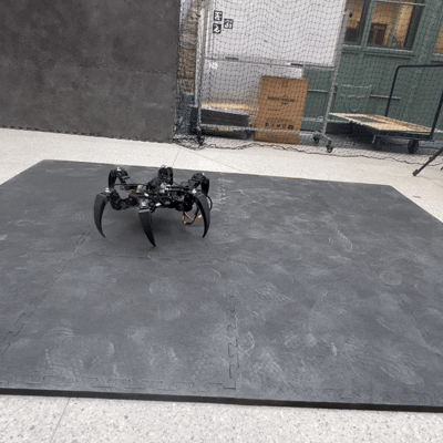
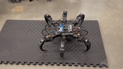
Look at him go!
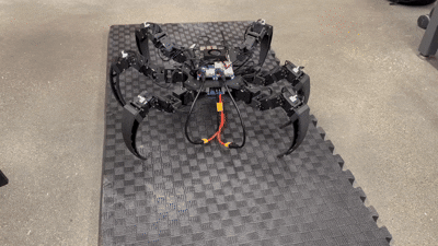
Greetings :)
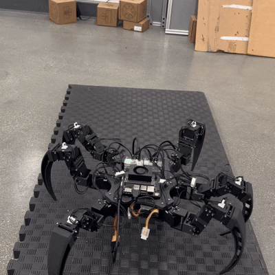
I started this project by creating a CAD model through several prototype iterations of legs and bases. The Hexapod uses Inverse kinematics for each of the legs to move in a 3 dimensional space. The current gait applied to its walking is the Tripod Gait, which is a popular and common gait for six legged animals. After creating the ability for the Hexapod to walk and turn, I trained a Reinforcement Learning algorithm to learn a gait that optimizes the linear velocity in the x direction. This algorithm is the Proximal Policy Optimization Algorithm, which is very popular in legged locomotion.
Hardware
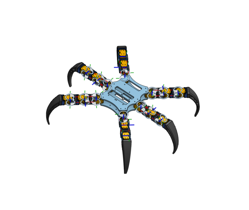
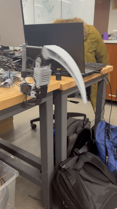
Hexapod CAD model
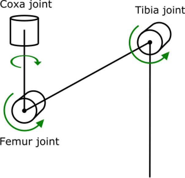
Leg Component Diagram
The CAD model consists of six legs, a top base, and a bottom base. I started by creating a single leg, which took many iterations to be successful. Each leg contains three motors, for the coxa, femur, and tibia respectively. The coxa motor turns about the z-axis meaning it moves the leg on the x-y plane. On the other hand (or leg I should say), the femur and tibia motors turn about the x-axis, meaning they move on the y-z plane. By using revolute mates, I could simulate these rotations. This would be especially useful for later when I train a RL model (which Ill need a URDF for).
Inverse Kinematics
IK with a Single Leg
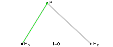
Bezier Curve for Leg Movement
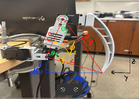
IK labels
To solve the IK, I started by looking at the first servo closest to the base that rotates
about the z-axis.
From a top-down view, we can calculate theta1. Since we know this servo operates on the x-y
plane it doesnt depend on the
other servos this is the easiet to solve.
The other two servos are a little more tricky. The drawing above lists the parameters that
are needed based on the leg,
and the full calculations are below. With this working, I can now move any leg to an
absolute x,y,z point in its workspace.
\begin{align} y &\leftarrow y + Y_{REST} \\ z &\leftarrow z + Z_{REST} \end{align}
\begin{align} \theta_1 &= \arctan\left(\frac{x}{y}\right) \cdot \frac{180}{\pi} \end{align}
\begin{align} r_1 &= \sqrt{x^2 + y^2} - R_1 \\ r_2 &= z \\ d &= \sqrt{r_1^2 + r_2^2} \end{align}
\begin{align} \phi_1 &= \arctan\left(\frac{z}{r_1}\right) \cdot \frac{180}{\pi} \\ \phi_2 &= \arccos\left(\frac{R_2^2 + d^2 - R_3^2}{2 \cdot R_2 \cdot d}\right) \cdot \frac{180}{\pi} \\ \phi_3 &= \arccos\left(\frac{R_2^2 + R_3^2 - d^2}{2 \cdot R_2 \cdot R_3}\right) \cdot \frac{180}{\pi} \end{align}
\begin{align} \theta_2 &= \phi_1 + \phi_2 \\ \theta_3 &= \phi_3 - 90 \end{align}
Tripod Gait
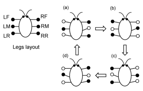
Tripod Gait Example
Tripod Gait in Action
Turning Using an "Inverted" Tripod Gait
A tripod gait is a walking pattern commonly used by six-legged insects and robots.
The name comes from the fact that the animal or robot maintains stability by keeping at
least three legs in contact with the ground at all times, forming a stable tripod.
The tripod gait is particularly efficient for fast movement across relatively flat terrain.
After achieving the tripod gait, others gaits and turning in place becomes trivial. For
example, now
the robot can by making only one change. Reverse the direction that the center legs move,
and now the hexapod turns!
Reinforcement Learning
Genesis RL Simulation
To successfully implement RL to optimize my gait and to teach the hexapod, I first needed to
export my
CAD model as a URDF to simulate each joint. This turned out to be a pain, but eventually
using onshape-to-robot got
it done. I then needed to choose a simulation platform. One of my cohort mates reccomended a
new
simulation platform called Genesis, which could be used to train legged locomotion policies
(perfect for my use case!).
Luckily, they had an example of training the unitree go2 robot dog, which also had 3 joints
per leg. So it took minimal
adjustment to successfully train and deploy an algorithm to teach my hexapod how to walk.
The algorithm used is the PPO (Proximal Policy Optimization) algorithm. In a nutshell,
This algorithm takes in the observation space as an input to a neural network, and outputs
a probability of likely actions to maxmize the reward. There is also another network that
has the
same input, and output the likely reward to be receieved. This Actor-Critic relationship
trains the hexapod
to walk!
-
Initialize Parameters:
- Initialize the policy network (actor) and value network (critic) with random weights.
- Set hyperparameters: learning rate, clipping range (\(\epsilon\)), discount factor (\(\gamma\)), GAE parameters (\(\lambda\)), etc.
-
Collect Trajectories:
- Use the current policy to interact with the environment and collect trajectories (states, actions, rewards, next states, and done flags).
-
Compute Advantages and Returns:
- Compute the discounted returns for each timestep using the rewards.
- Compute the advantages using Generalized Advantage Estimation (GAE) or another method.
-
Update Policy and Value Function:
- Compute the policy loss using the clipped surrogate objective: \[ L^{CLIP}(\theta) = \mathbb{E}_t \left[ \min \left( r_t(\theta) \cdot A_t, \text{clip}(r_t(\theta), 1-\epsilon, 1+\epsilon) \cdot A_t \right) \right] \]
- Compute the value function loss (mean squared error between predicted and actual returns).
where \( r_t(\theta) = \frac{\pi_\theta(a_t|s_t)}{\pi_{\theta_{\text{old}}}(a_t|s_t)} \) is the probability ratio.

DANCE!